 Djinious



Stochastic & quant finance
Simulation driven by randomness — Brownian motion, stochastic differential equations and Monte Carlo. Option prices that converge to Black–Scholes, variance reduction, path-dependent exotics, the Greeks, Value-at-Risk, and a volatility smile: the stochastic-calculus paradigm nothing else in the portfolio touches.
 DjiniousLab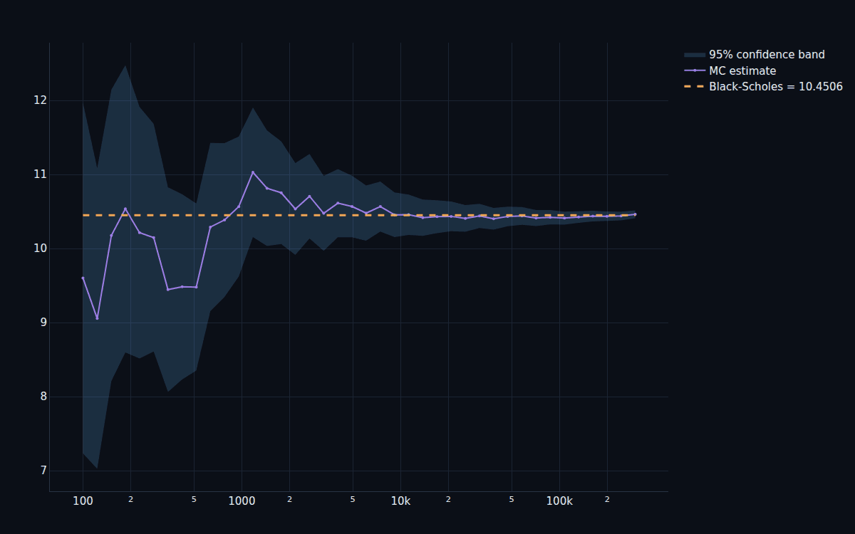
- Monte-Carlo vs Black–Scholes price
- <0.5%Monte-Carlo vs Black–Scholes price
- convergence rate (log–log slope)
- −0.50convergence rate (log–log slope)
- variance reduction (fewer paths, same accuracy)
- 2.6×variance reduction (fewer paths, same accuracy)
- put–call parity & Greeks match
- exactput–call parity & Greeks match
- design notebooks
- 10design notebooks
- requirements PASS
- 5 / 5requirements PASS
When the future is a distribution, you simulate it.
Every other model in this portfolio is deterministic: same inputs, same answer. But a stock price, a portfolio's loss, an option's payoff — these are random, and you can't integrate your way to them. You simulate thousands of possible futures and average. This program builds that stochastic paradigm — Brownian motion, stochastic differential equations, Monte Carlo — on its canonical application, quantitative finance: pricing options and measuring risk, anchored to the one case where a closed-form answer exists so the simulation can be trusted everywhere it doesn't.
A stock price is a random walk with drift.
Geometric Brownian motion — the foundation of quantitative finance — is a stochastic differential equation: a deterministic drift plus a random kick scaled by volatility, integrated with the Euler–Maruyama scheme. Simulate it many times and the paths fan out into a cone, their endpoints forming the lognormal distribution that underlies option pricing. This is the raw material: not one trajectory, but an ensemble of possible futures.
DjiniousLab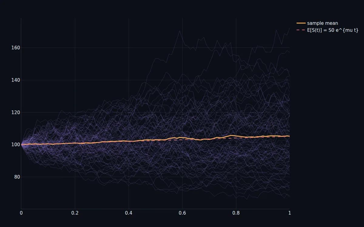 DjiniousLab
Accuracy costs paths — unless you're clever.
Monte-Carlo error shrinks only as 1/√N, so each extra digit of accuracy costs a hundred times the paths — the central tax of stochastic simulation. Variance-reduction techniques beat it: antithetic variates and control variates reach the same accuracy with a fraction of the paths (a 2.6× standard-error cut here, worth nearly 7× the work). Knowing these tricks is the difference between a Monte-Carlo pricer that's usable and one that isn't.
DjiniousLab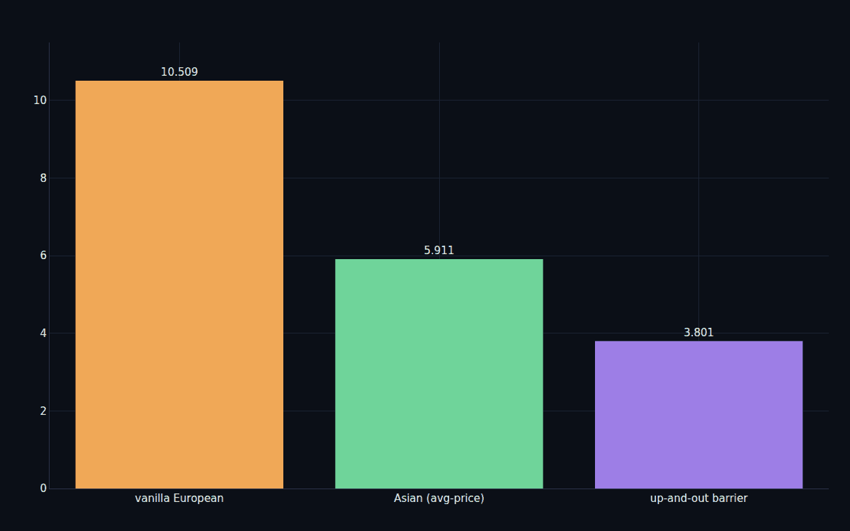
The same engine measures how much you could lose.
Turn the simulation on a portfolio instead of a single option and it produces a distribution of profit and loss — and from its tail, the risk numbers regulators and risk desks live by: Value-at-Risk (the loss you won't exceed 95% or 99% of the time) and Expected Shortfall (the average loss when you do). The program computes both, and contrasts a Gaussian Monte-Carlo tail against a fat-tailed historical one — the difference that decides whether a risk model sees the crash coming.
DjiniousLab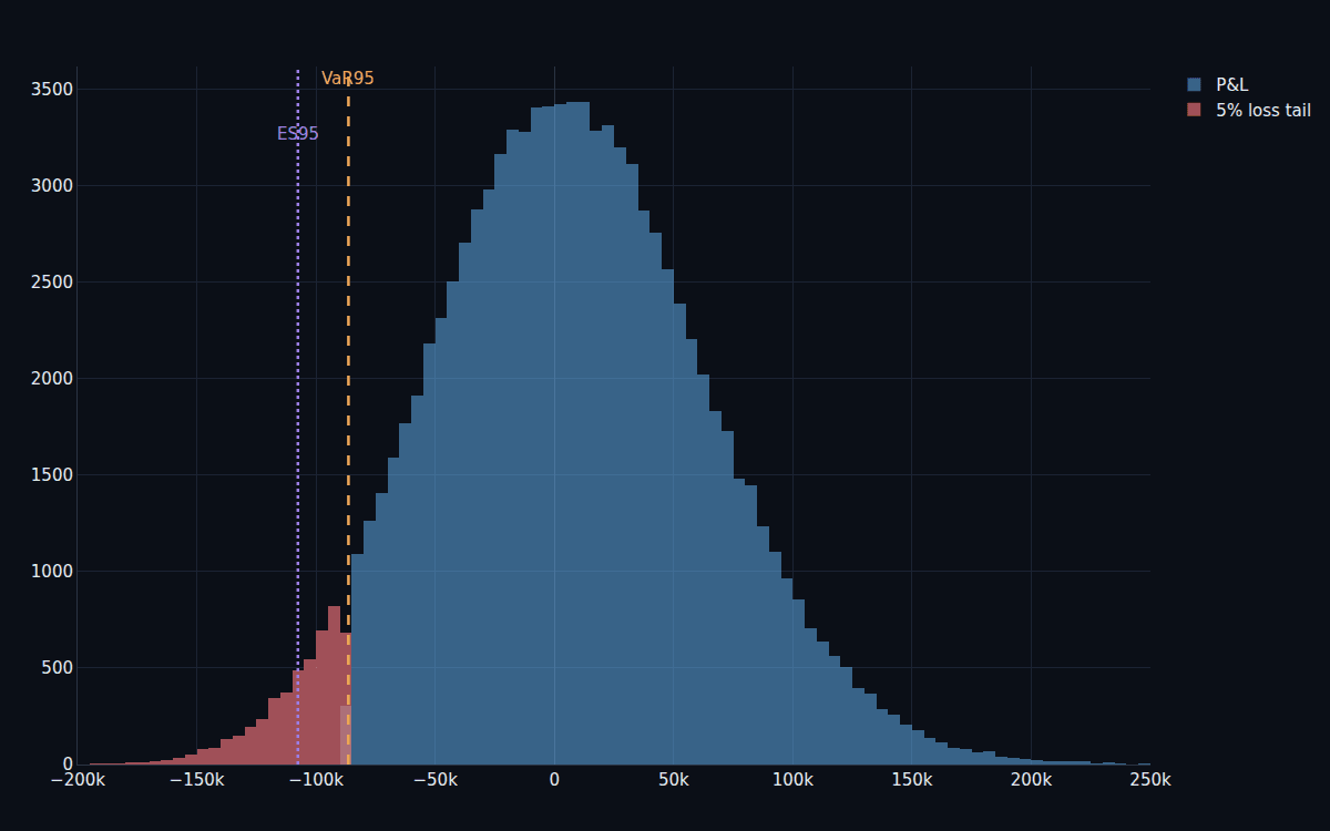
Real markets don't have one volatility.
Black–Scholes assumes a single constant volatility; real option markets don't, and the evidence is the volatility smile — implied volatility that varies with strike. A stochastic-volatility model (Heston), where volatility is itself a random process correlated with price, reproduces it: simulate the coupled processes and the implied-volatility curve skews and the return distribution grows a fat left tail that flat Black–Scholes misses. Stochastic simulation reaching what closed forms can't.
DjiniousLab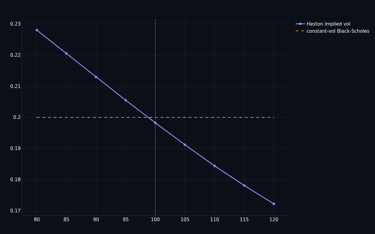
Every number re-derived at sign-off.
The V&V notebook rebuilds each estimator from scratch with fixed seeds and re-derives the requirements against theory, printing a PASS/FAIL board.
Result
- MC call vs Black–Scholes: 10.50 vs 10.45
- Convergence rate (log–log): −0.503
- Variance reduction (control variate): 2.6×
- Put–call parity / delta: exact / <0.01%
- VaR95 / ES95 ($1M book): $86k / $108k
Requirement
- MC call vs Black–Scholes: R-01 ≤ 2·SE
- Convergence rate (log–log): R-02 ≈ −½
- Variance reduction (control variate): R-03 ≥ 2×
- Put–call parity / delta: R-04
- VaR95 / ES95 ($1M book): R-05
A stochastic paradigm, anchored to theory.
The deliverable is ten notebooks and the dossier — stochastic paths and Monte-Carlo estimators, not an acausal network, so there's no custom block or canvas. The SDEs use the Euler–Maruyama scheme (not higher-order or exact schemes), the base process is constant-parameter geometric Brownian motion, pricing is risk-neutral, path counts are modest for notebook speed, and nothing is calibrated to real market data — the risk numbers are illustrative, not production. What the program proves is the paradigm itself: that the platform simulates stochastic systems, not just deterministic ones — validated against Black–Scholes where a closed form exists, and reaching path-dependent options, tail risk, and stochastic volatility where none does.
Keep exploring
Related use cases
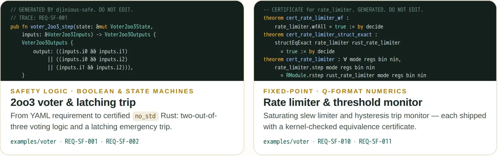 Safety-critical embedded controlNine safety functions, from YAML requirement to certified embedded RustThe voter reference project takes nine safety functions — voting, latching, slew limiting, trip monitoring, interlocks and a flow gauge with a floating-point boundary — through all thirteen gates, and replays every one on an emulated Cortex-M4F.
 DjiniousSafe
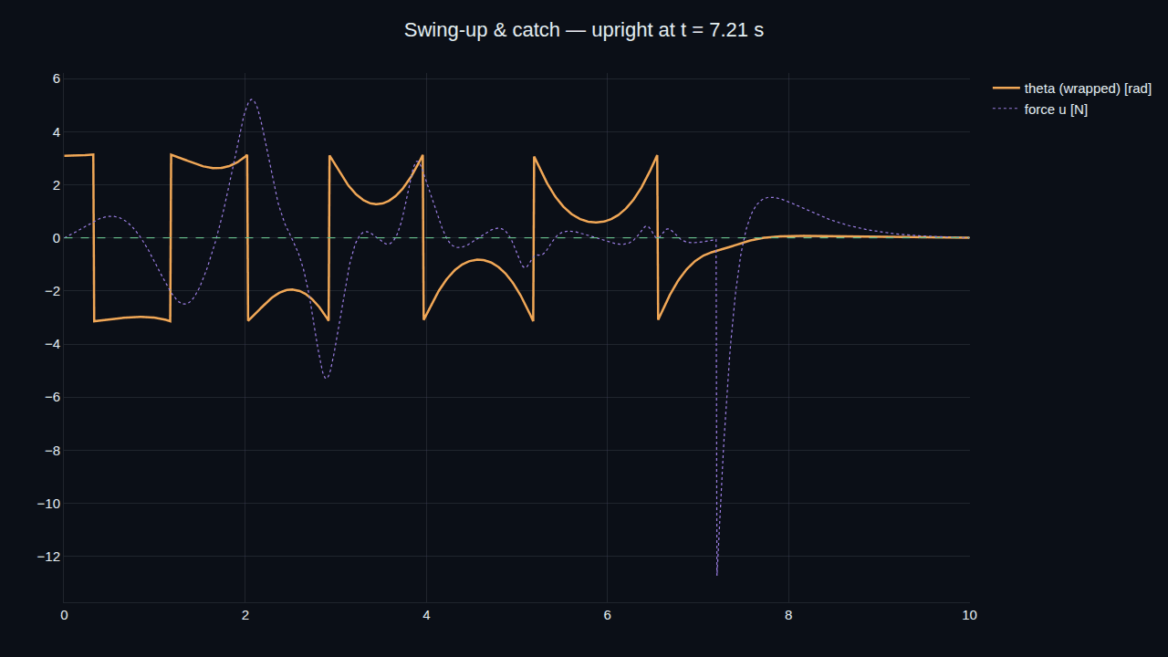 Control & reinforcement learningCart-pole control & RLThe canonical underactuated-control benchmark, taken end to end — nonlinear dynamics, an LQR that stabilises the inverted pole, energy swing-up, a model-free reinforcement-learning policy, and a Monte-Carlo robustness gate.DjiniousLab
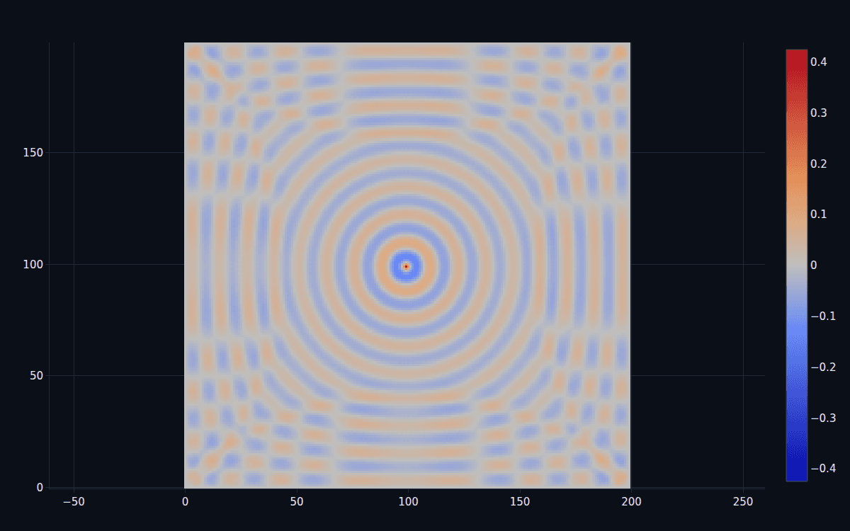 ElectromagneticsElectromagnetics (FDTD)Solving Maxwell's equations on a grid — the electric and magnetic fields leapfrogging through space and time. A self-contained FDTD solver reproduces the canonical wave phenomena: radiation, refraction, diffraction, scattering and cavity resonance. The field-solver sibling to CFD, in electromagnetics.DjiniousLab