 Djinious




Heat pump
A vapor-compression heat pump on the refrigerant cycle — the P-h diagram, compressor and heat exchangers, the COP and its Carnot limit, how COP falls with temperature lift, and the seasonal SCOP that beats resistance heat fourfold.
 DjiniousLab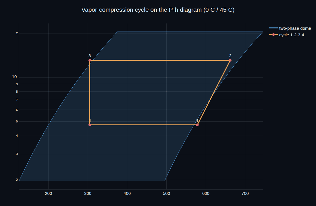
- COP at 0 °C → 45 °C
- 4.27COP at 0 °C → 45 °C
- of the Carnot limit
- 60%of the Carnot limit
- seasonal SCOP
- 3.70seasonal SCOP
- less electricity vs resistance
- 3.7×less electricity vs resistance
- balance point
- −2 °Cbalance point
- design notebooks
- 10design notebooks
One unit of electricity, four of heat.
A heat pump doesn't make heat — it moves it, and that's why it can deliver three to four units of warmth per unit of electricity. The trick is a refrigerant boiling and condensing around a loop. This program models the vapor-compression cycle on the pressure-enthalpy diagram, follows it through the compressor and heat exchangers, and answers the questions that decide a system: how high a COP, how far it falls in the cold, and what it actually averages over a heating season.
Boil low, condense high.
The refrigerant evaporates at low pressure, pulling heat from the cold outdoor air; the compressor squeezes it to high pressure; it condenses indoors, dumping that heat plus the compressor work; and an expansion valve drops it back to low pressure to start again. Drawn on the pressure-enthalpy diagram, the cycle is a rectangle riding the two-phase saturation dome, and every performance number — heat delivered, work in, coefficient of performance — is a width on that chart. At a 0 °C source and a 45 °C sink the cycle returns a COP of 4.27, about 60% of the reversible Carnot bound.
DjiniousLabCOP falls exactly when you need it most.
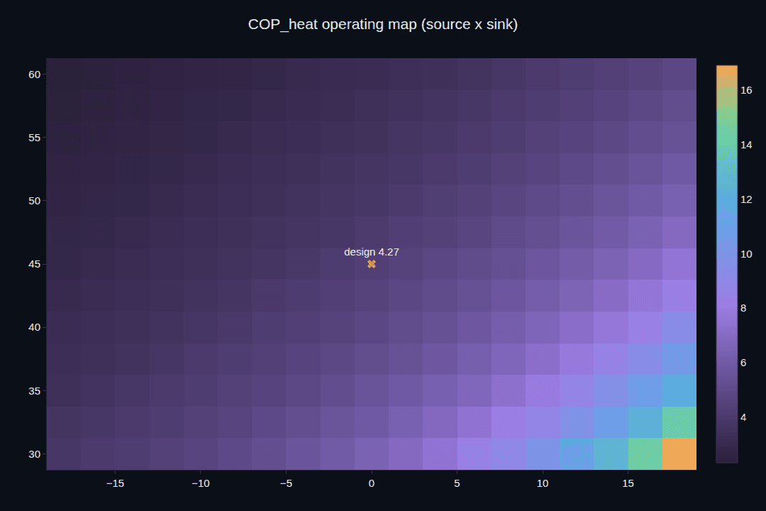
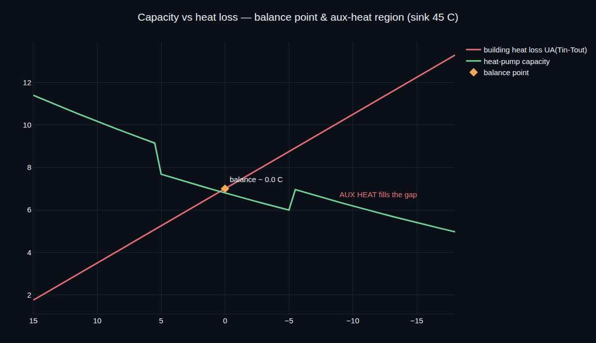
A heat pump's efficiency depends on the temperature lift — how far it has to pump heat uphill. On a mild day, lifting from 5 °C to a 45 °C flow, COP is near five. On a cold one, lifting from −15 °C, it drops to three, because the same compressor faces a far larger pressure ratio. That's the central design tension: demand is highest when efficiency is lowest. The program traces COP across the whole source-and-sink envelope, finds the balance point where capacity meets the building's heat loss (around −2 °C here), and shows where a backup is needed — the analysis that sizes a real installation.
DjiniousLab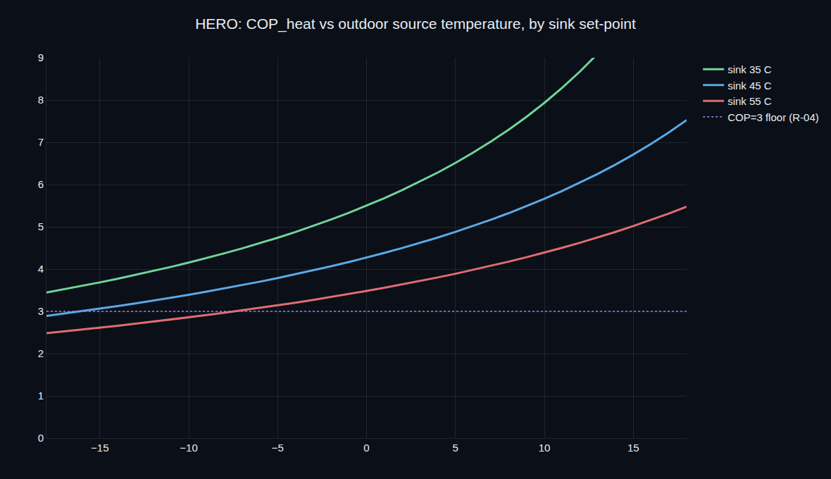 DjiniousLab
 DjiniousLab
 DjiniousLab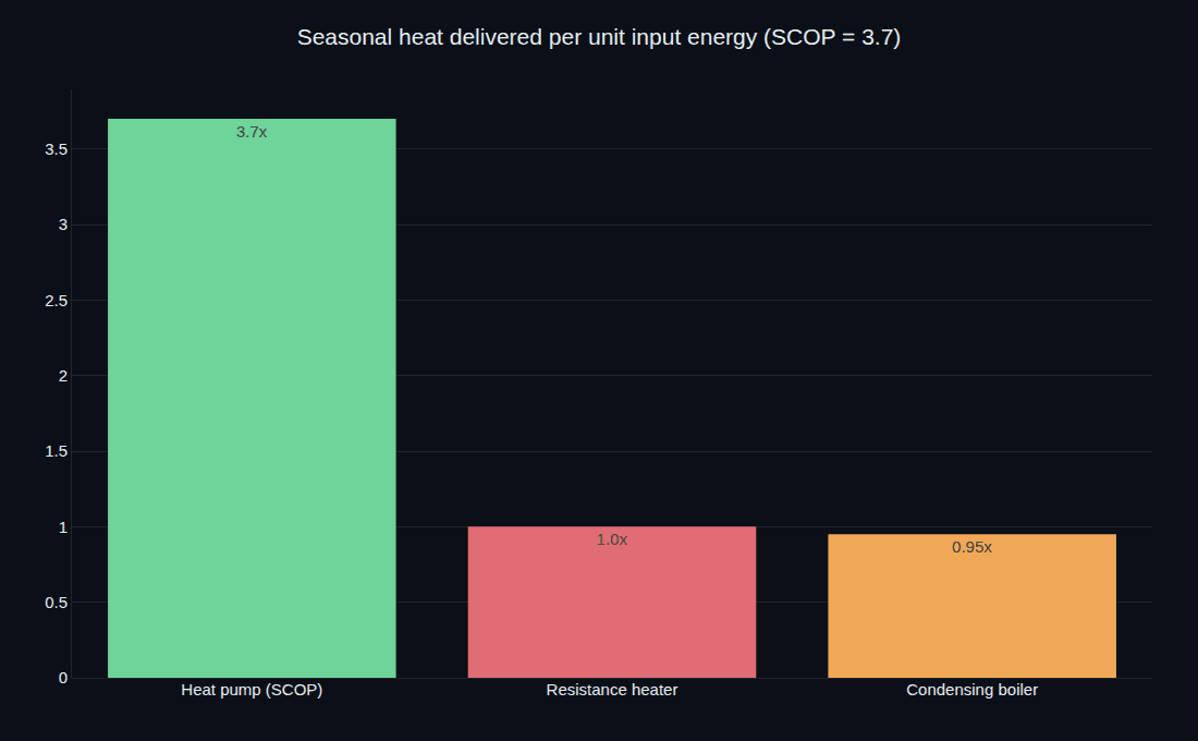
Every number is one you can re-run.
The sign-off notebook re-derives each requirement from the same cycle the program builds.
Result
- COP @ 0 °C / 45 °C: 4.27
- Second-law efficiency: 60.4%
- COP @ −15 °C source: 3.06
- Seasonal SCOP: 3.70
- Requirements verified: 6 / 6
Requirement
- COP @ 0 °C / 45 °C: ≥ 4.0
- Second-law efficiency: ≥ 50%
- COP @ −15 °C source: ≥ 3.0
- Seasonal SCOP: ≥ 3.5
- Requirements verified: PASS
Idealized refrigerant, real cycle.
The refrigerant is an idealized R290 — Clausius-Clapeyron saturation pressure with constant latent heat and specific heats, not a CoolProp/REFPROP equation of state — which keeps every number reproducible and the physics teachable. The cycle is steady thermodynamics, not a dynamic component model; the compressor is an isentropic-efficiency block; the SCOP is a temperature-bin method, not a full EN 14825 rating. That is exactly the fidelity a heat-pump concept and sizing study needs first — choosing the refrigerant and pressures, mapping COP against climate, finding the balance point, and trading supply temperature against efficiency — on your own numbers, before a manufacturer's detailed model.
Keep exploring
Related use cases
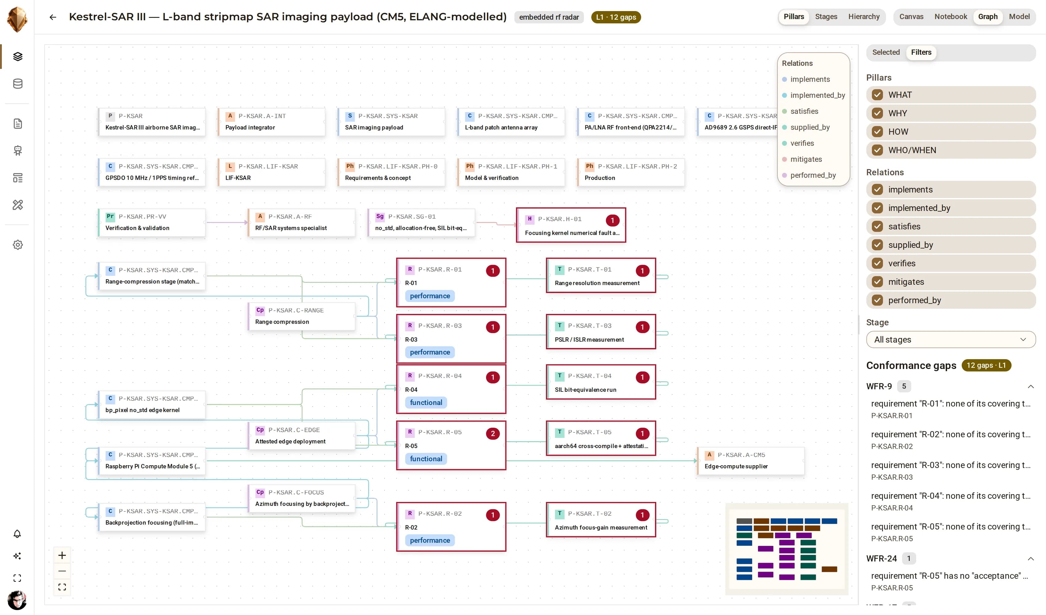 Grid-scale energySunnyGrid80 Solar-Storage PlantAn 80 MW photovoltaic plant with a 40 MW / 80 MWh battery energy-storage system and its grid substation, modelled in ELANG as an audited reference to UL 9540A and IEC 62443 — a system-of-systems where the interfaces carry as much of the design as the boxes.
 DjiniousEngineering
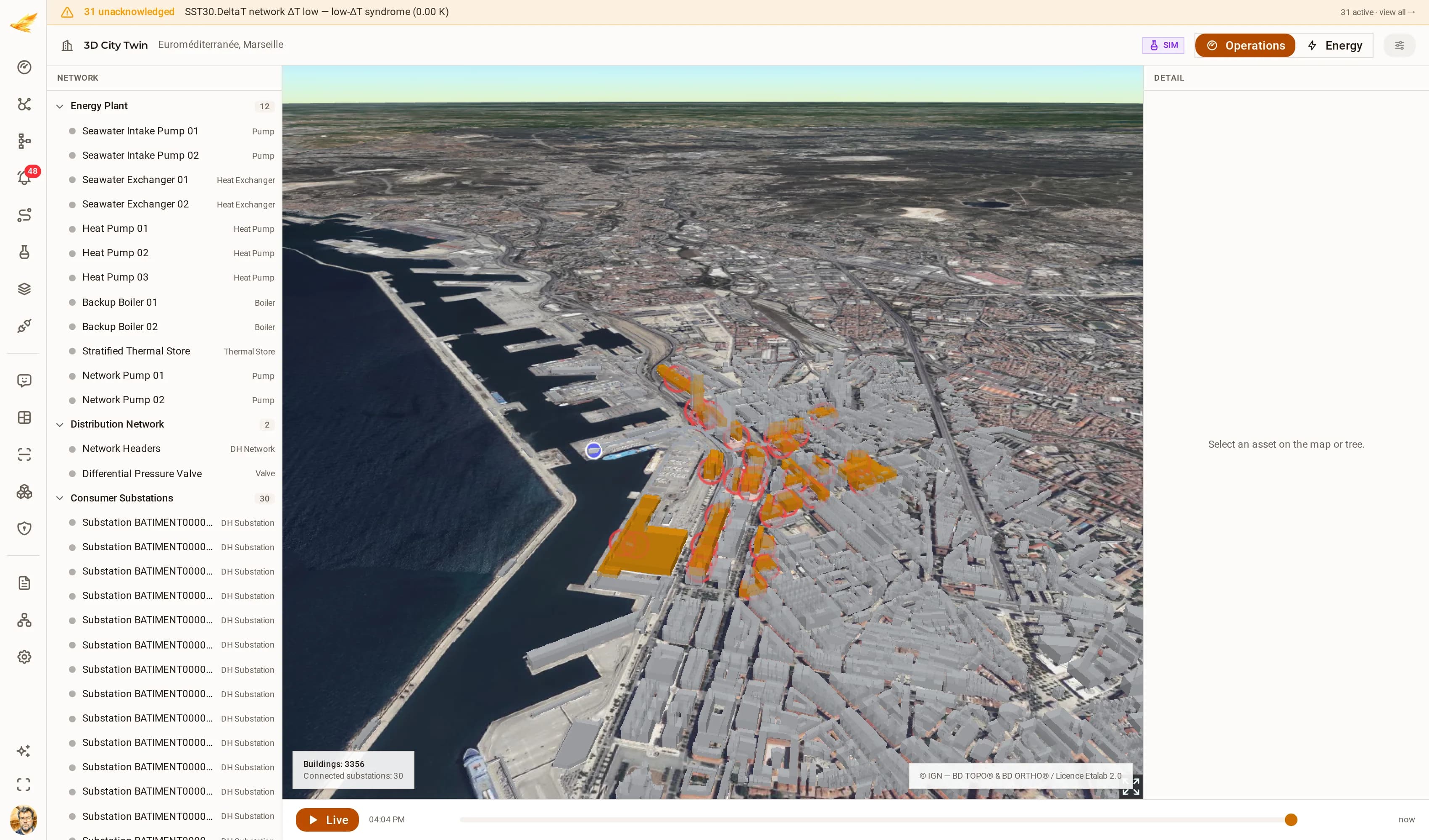 District energyEuroméditerranée District Energy NetworkA seawater-source district-heating network: two intake pumps and two seawater exchangers feeding three heat pumps, two backup boilers and a stratified thermal store, distributing through two network pumps and a differential-pressure valve to thirty consumer substations. The network is simulated; the city under it is not — every substation sits on its real IGN BD TOPO® building footprint in the Euroméditerranée quarter. It is a demonstration network on open data, not any operator's plant.
 DjiniousCC
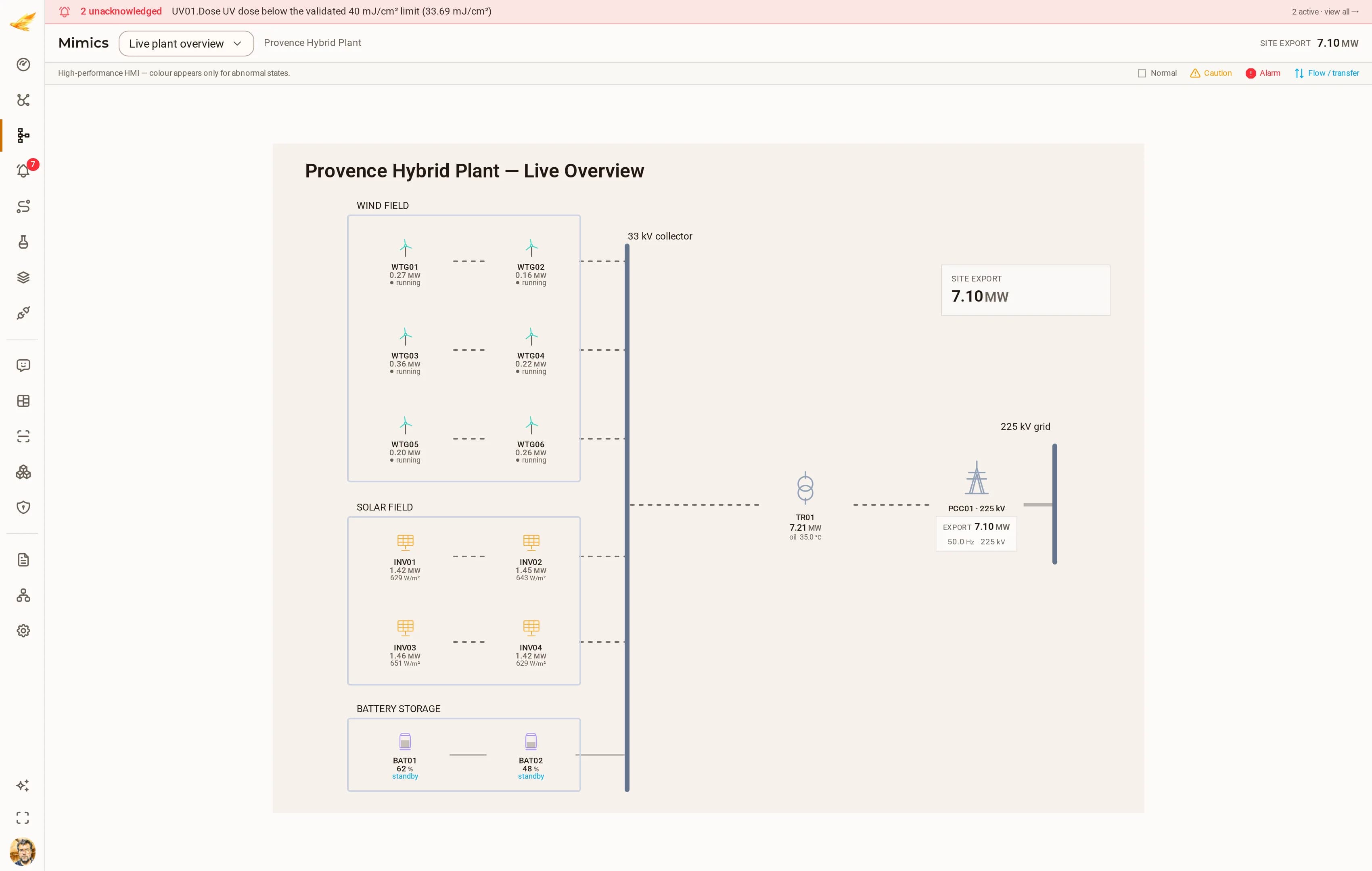 Renewable generationProvence Hybrid PlantA 120 MW hybrid plant: six wind turbines, four PV inverter blocks, two battery racks, the main 33/225 kV transformer, the grid connection point and a meteorological mast.DjiniousCC